In April of this year, IBM released the latest version of SPSS Statistics. Version 26 introduces a number of additional analysis procedures as well as new command enhancements. If you’re an existing SPSS user and you’d like to upgrade to v26 there’s more information about how to do that here. If you’re interested in trying SPSS Statistics for the first time then do please get in touch – we’ll be happy to help.
New analytical procedures
Quantile Regression
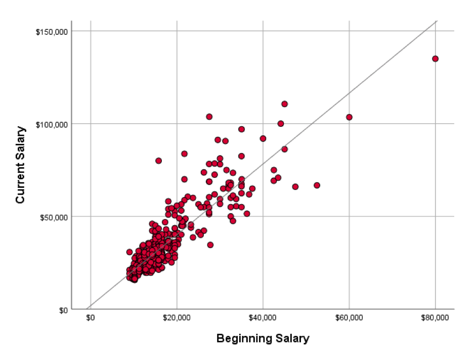
In standard ‘least squares’ regression the model predictions are based on a single regression line. This line can be used to estimate the mean value of the dependent variable as represented by the points clustering about line at a given value of the independent (predictor) variable (see figure 1)

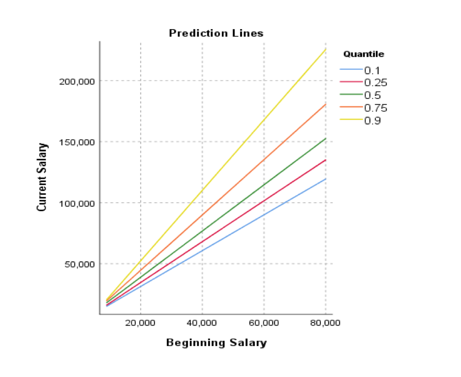
You may note from the chart that there seems to be a slight ‘funnelling’ of the points near the higher values in the scatterplot. Technically, this is referred to as ‘heteroscedasticity’, but more prosaically, it just indicates that the model is likely to be worse at estimating higher values than lower ones since the points vary more about the line. Quantile regression offers us the opportunity to fit the model using a median value rather than a mean. We should bear in mind that a median is also called the 50th percentile and in this context percentile and quantile refer to the same thing. Although there’s no reason to believe that a regression based on line fitted about the median would be more accurate than one based on a mean, quantile regression is flexible enough to allow us to fit a model based on other percentile values. In other words, we can fit separate regression lines for different percentiles. For example, we can request estimates for the lowest 10 percent (quantile = 0.1) or the top 90 percent (quantile = 0.9) of the dependent variable.

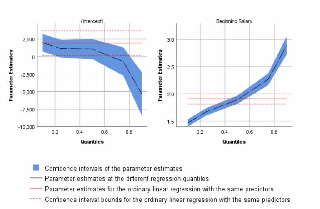
The effect of this is that we can produce separate predictions for the different parts of the dependent variable’s distribution. Using standard Linear Regression on the same dataset we get a single formula for estimating a respondent’s current salary. This formula consists of a single coefficient of 1.9, meaning that for every extra dollar of beginning salary, the respondent earns $1.9 dollars in their current salary. The formula also contains a constant value (or intercept) of $1,928. However, there’s no reason to assume that the same formula applies to the data in the top 10% of the current salary distribution, or the say, the bottom 25%. As such, Quantile regression produces separate coefficients and intercept values for each requested quantile. The new Quantile regression procedure even plots these values as shown in figure 3.

The charts even show the parameter values for a standard (OLS) linear regression model for comparison (as indicated by the red line). Figure 3 illustrates that not only do we get different intercept values for data in the 20th percentile (quantile 0.2) vs the 80th percentile (quantile 0.8), but we also get different parameter estimates for the coefficient values.
ROC Analysis
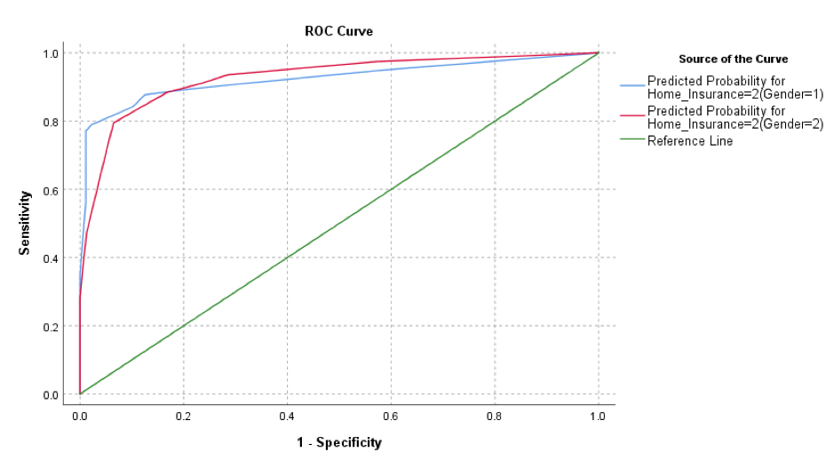
The new ROC procedure makes it easier to assess the accuracy and performance of predictive classification models. ROC (Receiver Operator Characteristic) analysis is specifically concerned with the classification accuracy of models, especially as regards the relationships between the accurate classifications (known as the True Positives and True Negatives) and the inaccurate predictions (the False Positives and False Negatives). These are often represented by a ROC curve that plots the true positive rate (TPR) against the false positive rate (FPR) at various threshold settings. The new ROC Analysis procedure also includes precision-recall (PR) curves and provides options for comparing two ROC curves that are generated from either independent groups or paired subjects.

Bayesian Statistics
SPSS Statistics v26 also includes enhancements to its suite of bayesian statistical procedures.
One-way Repeated Measures ANOVA
The repeated measures enhancement allows the analyst to adopt a Bayesian approach to comparing any changes in a given factor for the same subject at different time points or conditions. It is assumed that each subject has a single observation for each time point.
One Sample Binomial enhancements
Here the user may apply a Bayesian binomial test to attempt to determine the likelihood that the observed ratio between two groups are the same as an assumed proportion in the population.
One Sample Poisson enhancements
Like the previous procedure, except here the user may compare their data to how well it fits a Poisson distribution. These distributions are a useful modelling for rare events such as accidents or insurance claims. A conjugate prior within the Gamma distribution family is used when drawing Bayesian statistical inference on Poisson distribution.
Reliability Analysis
Some additional enhancements have been made to SPSS Statistics’ reliability procedures.
Reliability analysis has now been updated to provide options for Fleiss’ Multiple Rater Kappa statistics. This technique is often employed when assessing the reliability of agreement between a fixed number of raters when assigning categorical ratings to a number of items or classifying items. This contrasts with other kappa values (such as Cohen’s kappa) which only apply to assessments of agreement between a maximum of two raters.
Command enhancements
SPSS V26 also includes enhancements to syntax commands
MATRIX-END MATRIX command
Long variable names (up to 64 bytes) can be used to name a matrix or vector name (such as COMPUTE, CALL, PRINT, READ, WRITE, GET, SAVE, MGET, MSAVE, DISPLAY, RELEASE, and so on).
Variable names that are included in a vector or matrix object are truncated to 8 bytes. This is because the matrix/vector structure is an array of numbers, and each number can match a string only up to 8 bytes. Long names (up to 64 bytes) are supported only when explicitly specified.
Long variable names are supported in GET and SAVE commands when explicitly specified on the /VARIABLES subcommand (and when specified on the /STRINGSsubcommand for the SAVE command). Variable names for GET and SAVE commands are truncated to 8 bytes when they are referenced through a vector in the /NAMESsubcommand.
The GET, SAVE, MGET, or MSAVE statements support both dataset references and physical file specifications.
MATRIX-END MATRIX now supports statistical functions that were previously only supported by the COMPUTE command (for example IDF.CHISQ, CDF.NORMAL, NCDF.F, and so on).
GENLINMIXED command
New Covariance Type structures ARH1 & CSH, Random Effects. The CSH and ARH1 options were added to the /RANDOM subcommand (keyword COVARIANCE_TYPE).
New Covariance Type structures ARH1 & CSH, Repeated Effects. The CSH and ARH1 options were added to the /DATA_STRUCTURE subcommand (keyword COVARIANCE_TYPE).
Kenward – Roger Degree of Freedom method. The KENWARD_ROGER option was added to the /BUILD_OPTIONS subcommand (keyword DF_METHOD).
Kronecker Covariance types. The options UN_AR1, UN_CS, UN_UN were added to the /DATA_STRUCTURE subcommand (keyword COVARIANCE_TYPE).
New KRONECKER_MEASURES keyword. The keyword is used for specifying a list of variables for the /DATA_STRUCTURE subcommand. The keyword should be used only when COVARIANCE_TYPE is one of three Kronecker types. The rules for KRONECKER_MEASURES are the same as for REPEATED_MEASURES. When both specifications are in effect, they may or may not have common fields, but cannot be exactly the same (regardless of whether they are in the same order).
MIXED command
DFMETHOD keyword introduced on the CRITERIA subcommand.
KRONECKER keyword added to the REPEATED subcommand. The keyword should be used only when COVTYPE is one of three following Kronecker types.
UN_AR1, UN_CS, and UN_UN options added to the COVTYPE keyword on the REPEATED subcommand.

